
📚 Well Testing for Beginners — Part 3 of 5
What Is a Drawdown Test?
A drawdown test is a well test performed while the well is producing. The well starts from a shut-in condition (no flow, stable pressure) and is then opened to flow at a constant rate. Engineers measure how the bottomhole pressure drops over time as fluid drains from the reservoir.
The name “drawdown” refers to the pressure being drawn down (reduced) from its initial value as the well produces. It is the complement of the buildup test — instead of watching pressure rise after shut-in, you watch it fall after the well opens. See Pressure Buildup Test for the companion test.
Drawdown vs. Buildup: What’s the Difference?
Both tests give similar information, but they have different practical advantages:
A drawdown test works best at the very beginning of a well’s life, before it has produced much. If the well starts from a known initial reservoir pressure, the analysis is straightforward. The drawback is that it’s very hard to hold flow rate perfectly constant — any variation affects the pressure data and complicates analysis.
A buildup test is easier to perform because shutting a well in is simpler than controlling a constant flow rate. This is why buildup tests are more common in everyday field operations. However, buildup tests require a known producing history before shut-in.
If you are new to well testing, start with What Is Well Testing? for the full context before diving into test types.
The Three Flow Regimes
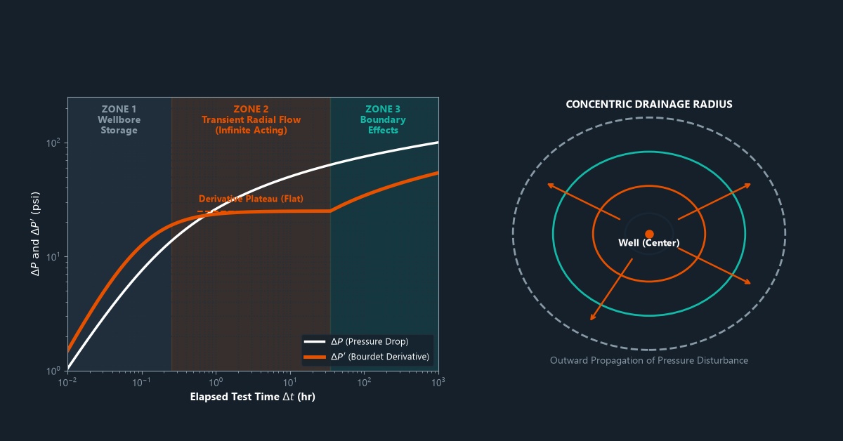
When a well starts producing, the pressure disturbance moves outward through the reservoir in stages. Each stage is called a flow regime. Understanding flow regimes is fundamental to interpreting any well test.
1. Early Time Region (ETR) — Wellbore Storage and Skin
At the very start of production (or shut-in), the pressure response is dominated by wellbore storage — the compression or expansion of fluid already inside the wellbore itself. The reservoir has not yet “felt” the disturbance. During this period, the data doesn’t reflect true reservoir properties and is typically excluded from analysis.
On a log-log plot, the ETR shows up as a straight line with a slope of 1 (called a “unit slope line”). The duration of wellbore storage depends on the wellbore volume and the formation properties.
2. Middle Time Region (MTR) — Infinite-Acting Radial Flow
Once the pressure disturbance moves past the wellbore storage period, the reservoir enters infinite-acting radial flow (IARF). In this regime, the pressure wave travels outward in all directions like an expanding ripple on a pond. The reservoir behaves as if it has no boundaries — it appears “infinite” to the pressure signal.
This is the most important regime for analysis. The middle time region (MTR) is where the Horner plot straight line forms, and from which permeability and skin are calculated. On the log-log derivative plot, IARF appears as a flat (horizontal) line in the derivative at a value of 0.5 × ΔP (using the standard convention).
The skin factor calculated from this region tells you whether the well is damaged or stimulated.
3. Late Time Region (LTR) — Boundary Effects
Eventually, the pressure wave reaches the outer boundaries of the reservoir — faults, edges, or other barriers. The reservoir can no longer act as infinite. This is the late time region (LTR), and the pressure behavior changes depending on what type of boundary is present.
A sealing fault doubles the slope on the semilog plot (the derivative rises to a new flat level on the log-log plot). The fault reflects the pressure signal back.
A constant-pressure boundary (like a large aquifer) causes the pressure to stabilize — the derivative drops on the log-log plot as the boundary supplies pressure support.
A closed reservoir shows a rising derivative at late time as pressure depletion becomes apparent across the whole reservoir.
Special Flow Regimes
Beyond the three main regimes, some reservoirs show additional flow patterns that give extra information:
Linear Flow
When fluid flows in parallel lines rather than radially — for example, toward a hydraulic fracture — the well shows linear flow. On a log-log plot, the derivative has a slope of 0.5 during linear flow. This is very common in hydraulically fractured wells and is used to calculate the fracture half-length. See Hydraulic Fracturing Overview for more on fractures.
Bilinear Flow
In a finite-conductivity fracture, fluids flow in two simultaneous linear patterns — along the fracture and from the reservoir into the fracture. This is bilinear flow, and on a log-log plot it shows a derivative slope of 0.25 (or a quarter-unit slope). It is used to calculate fracture conductivity.
Spherical Flow
When only part of the reservoir thickness is perforated, fluid flows in a spherical pattern toward the perforations. Spherical flow shows up as a slope of −0.5 on the derivative. This occurs in partially penetrating wells or when perforations are limited to a short interval. Learn more about perforation in oil wells.
How Is Drawdown Data Analyzed?
The traditional method plots the flowing bottomhole pressure versus the log of time. During the MTR, this produces a straight line. The slope of this line is used to calculate permeability with the same formula as the buildup test — but using different time and pressure variables.
Modern analysis uses the same log-log derivative approach as described for buildup tests. The derivative of the pressure drop (dΔP/d ln t) is plotted versus time, and the diagnostic shapes identify which flow regimes are present and in what order. Understanding key pressure definitions is essential before starting any analysis.
Frequently Asked Questions
Why is constant rate so important in a drawdown test?
The analysis equations assume a constant flow rate. If the rate changes during the test, the pressure response becomes a combination of multiple signals, making analysis much harder. Rate changes create “kinks” in the pressure curve that can be mistaken for reservoir features. Modern software can account for variable rates using superposition, but constant-rate tests are always simpler to analyze.
What is the investigation radius?
The investigation radius (or radius of investigation) is how far into the reservoir the pressure signal has traveled by a given time. It is estimated as: r_i ≈ 0.032 × √(k × t / (φ × μ × ct)) in field units. Longer tests investigate farther into the reservoir and can detect boundaries or heterogeneities at greater distances. The reservoir’s permeability directly controls how fast the signal travels.
Summary
The drawdown test captures reservoir behavior as a well flows for the first time. By identifying the three flow regimes — early time (wellbore storage), middle time (radial flow), and late time (boundary effects) — engineers build a detailed picture of the reservoir without leaving the surface. Special flow regimes like linear and bilinear flow reveal the presence and properties of fractures.
Next, we will look at a test specifically designed for new wells before they are completed: the Drill Stem Test (DST).
➡️ Next in this series: Drill Stem Test (DST): Testing Before Completion


Leave a Reply